Friday, August 15, 2014

Week Eight: "Linearity Property & Source Transformation"


What is a Linearity Property? 

Linearity is the property of an element describing a linear relationship between cause and effect. Although the property applies to many circuit elements, we shall limit its applicability to resistors in this chapter. The property is a combination of both the homogeneity (scaling) property and the additivity property. The homogeneity property requires that if the input (also called the excitation) is multiplied by a constant, then the output (also called the response) is multiplied by the same constant. For a resistor, for example, Ohm’s law relates the input i to the output v,


V= iR.

If the current is increased by a constant k, then the voltage increases correspondingly by k, that is,


kiR = kV

 The additivity property requires that the response to a sum of inputs is the sum of the responses to each input applied separately. Using the voltage-current relationship of a resistor, if


V1 = i1R
and
V2 = i2R 

then applying (i1+i2) gives,

V = (i1+i2)R = i1R + i2R = V1 + V2

We say that a resistor is a linear element because the voltage-current relationship satisfies both the homogeneity and the additivity properties.

In general, a circuit is linear if it is both additive and homogeneous. A linear circuit consists of only linear elements, linear dependent sources, and independent sources.


A Linear Circuit is one whose output is linearly related (or directly proportional)  to its input.


Example:


What is a Source Transformation?

We have noticed that series-parallel combination and wye-delta transfor-mation help simplify circuits. Source transformation is another tool for simplifying circuits. Basic to these tools is the concept of equivalence.

We recall that an equivalent circuit is one whose v-i characteristics areidentical with the original circuit.

Before, we saw that node-voltage (or mesh-current) equa- tions can be obtained by mere inspection of a circuit when the sources are all independent current (or all independent voltage) sources. It is therefore expedient in circuit analysis to be able to substitute a voltage source in series with a resistor for a current source in parallel with a resistor, or vice versa. Either substitution is known as a source transformation.


Figure 1:
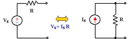

A Source Transformation is the process of replacing a voltage source Vs in series with a resistor R by a current source Is in parallel with a resistor R, or vice versa.

Source transformation requires that,

Vs = IsR     or     Is = Vs/R

Source transformation also applies to dependent sources, provided we carefully handle the dependent variable. As shown in below, a dependent voltage source in series with a resistor can be transformed to a dependent current source in parallel with the resistor or vice versa.

Figure 2:


Like the wye-delta transformation we studied in Chapter 2, a source transformation does not affect the remaining part of the circuit. When applicable, source transformation is a powerful tool that allows circuit manipulations to ease circuit analysis. However, we should keep the following points in mind when dealing with source transformation.

  1. Note from Fig.1 (or Fig.2) that the arrow of the current source is directed toward the positive terminal of the voltage source.
  2.  Note that source transformation is not possible when R=0, which is the case with an ideal voltage source. However, for a practical, nonideal voltage source, R=0. Similarly, an ideal current source with R=∞ cannot be replaced by a finite voltage source. 

Example:


Some Learnings:

  • Linearity Property talks about the voltage (v) and current (i), whereas voltage is directly proportional to the current, that is, when the voltage is increasing the current also increasing and vice  versa.
  • Source Transformation is only applicable to simple circuits like the figures below:


    but is not applicable to complicated circuits like figures below:

  • Source Transformation can be applied if and only if the voltage is in series with the resistor and/or the current is in parallel with the resistor.
  • In Source Transformation when the polarity of the voltage source has a positive on top therefore the resulting current source is pointing upward and vice versa. Also when the voltage source is dependent therefore the resulting current is also dependent, same goes with independent sources.
Videos:


For more information, watch the videos below:

For Linearity Property:


For Source Transformation:


That's all. Thank You for visiting my blog.
GOD Bless! :)


By:
AYALA, ARNY  S.   BSECE -3
ECE 311
Professor:
ENGR. JAY S. VILLAN, MEP - EE


Saturday, August 9, 2014

Week Seven: "Mesh Analysis"


What is a Mesh Analysis?


Mesh analysis provides another general procedure for analyzing circuits, using mesh currents as the circuit variables. Using mesh currents instead of element currents as circuit variables is convenient and reduces the number of equations that must be solved simultaneously. Recall that a loop is a closed path with no node passed more than once. A mesh is a loop that does not contain any other loop within it.
Nodal analysis applies KCL to find unknown voltages in a given circuit, while mesh analysis applies KVL to find unknown currents. Mesh analysis is not quite as general as nodal analysis because it is only applicable to a circuit that is planar. A planar circuit is one that can be drawn in a plane with no branches crossing one another; otherwise it is nonplanar. A circuit may have crossing branches and still be planar if it can be redrawn such that it has no crossing branches.

To understand mesh analysis, we should first explain more about what we
mean by a mesh.

In Figure below, for example, paths abefa and bcdeb
are meshes, but path abcdefa is not a mesh. The current through a mesh is
known as mesh current. In mesh analysis, we are interested in applying KVL to 
find the mesh currents in a given circuit.


In this section, we will apply mesh analysis to planar circuits that do not
contain current sources. In the next sections, we will consider circuits with 

current sources. In the mesh analysis of a circuit with n meshes, we take the 
following three steps.
Steps to Determine Mesh Currents:
  1. Assign mesh currents i1,i2,...,into the n meshes.
  1. Apply KVL to each of then meshes. Use Ohm’s law to express the
    voltages in terms of the mesh currents.
  1. Solve the resulting n simultaneous equations to get the mesh currents.

Mesh Analysis Without Current Sources:

Example:
 
Now write KVL equations for each loop.

@Mesh 1:
-18V + 5(i1-i2) + 4(i1-i3) + 1(i1) = 0
then gather terms:
10i1 - 5i2 - 4 i3 -18V = 0

Note that the i1 term is positive, and all other current terms are negative (because 
they are all clockwise, all other panes will contribute a negative term). Let's do the 
other two panes with terms gathered up directly (write the total resistance of the 
loop multiplied by the mesh current that goes through that total resistance):
@Mesh 2:
-5i1 + 10i2 - 3i3 - 12 = 0
@ Mesh 3:
-4i1 -3i2 +9i3 = 0
Now solve the three equations in three unknowns:
i1 = 7.02A
i2 = 6.28A
i3 = 5.21A

The current through the 5 ohm resistor is just i1 - i2, or 0.74A. The current 
through the 18V is i1, or 7.02A. All the branch currents are shown below from a 
Pspice simulation:


Mesh Analysis With Current Sources:

Applying mesh analysis to circuits containing current sources (dependent or independent) may appear complicated. But it is actually much easier than what 
we encountered in the previous section, because the presence of the current 
sources reduces the number of equations. Consider the following two possible 
cases.

Case 1:
When a current source exists only in one mesh. We set
mesh current i equal to that current source.

Case 2:
When a current source exists between two meshes. We create a supermesh 
by excluding the current source and any elements connected in series with 
it.


Examples:

Case1:

First, define a mesh current arround each mesh (window pane) of the circuit. 
Define each one in a clockwise direction.


Now write KVL equations for each loop. On the first loop, we run into a problem. 

We do not know the voltage across the 5A source. (This is one of the difficulties 
you can run into when using mesh current.) We add a new unknown to handle this problem. We run into the same problem with the 2A source, so two new unknowns 
 (V5 and V2) are labeled:


Now we are ready to write the KVL equations.

@Mesh 1:
-V5 + 5(i1-i2) = 0
@ Mesh 2:
5(i2-i1)+10(i2-i4)+2(i2-i3) = 0
or
-5i1 + 17i2 - 2i3 = 0

@Mesh 3:
2(i3-i2) + V2 = 0
@Mesh 4:
10i4 + 4V + 10(i4-i2) = 0
or
-10i2 + 20i4 = -4
We have two extra unknowns, so we need two more equations. These can be 
found by examining the loops with the sources:

i1= 5A
i3 = -2A
We can then solve for the remaining unknowns:

i2 = 1.58A
i4 = 0.59A

We can then find the current through the 5 ohm resistor as:

I = i1 - i2 = 3.42A

The current through the 4V source is simply i4, or 0.59A.


Case 2:


Determine the values of the mesh currents, i1and i2, for this circuit.

Solution:
We can write one mesh equation by considering the current source. The current
source current is related to the mesh currents at by

(KCL)
 i1 - i2 = 1.5  or  i1 = 1.5 + i2

In order to write the second mesh equation, we must decide what to do about the

current source voltage. (Notice that there is no easy way to express the current
source voltage in terms of the mesh currents.) In this example, illustrate two 
methods of writing the second mesh equation.

Apply KVL to the supermesh corresponding to
the current source. Shown below in
blue, this supermesh is the perimeter of the two meshes that each contain the
current source.

 
 @ Supermesh:
9i1 + 3i2 + 6i2 - 12 = 0   or   9i1 + 9i2 = 12

Solving the equations gives:
i1 = 1.4167A   and   i1 = -83.3mA

Some Learnings:
  • Mesh Analysis uses KVL to obtain unknown mesh currents, while Nodal Analysis uses KCL to obtain unknown nodal voltages.
  • Mesh Analysis is only applicable to planar circuits. Planar circuits are circuits that can be drawn on a plane surface, with no wires crossing each other.
  • Mesh Analysis is different from Loop Analysis. Loop Analysis is applicable to both planar or not. Both Mesh & Loop Analysis make use of Kirchhoff's 
  • Voltage Law or KVL.
  • Mesh Analysis is usually easier to use when the circuit is planar, compared to Loop Analysis.

Video:

       For more information, watch the video below:


That's all. Thank You for visiting my blog.
GOD Bless! :)


By:
AYALA, ARNY  S.   BSECE -3
ECE 311
Professor:
ENGR. JAY S. VILLAN, MEP - EE


Saturday, August 2, 2014

Week Six: "Wye - Delta Transformations"


What is Wye - Delta Transformations?

     This week we talked about Wye - Delta Transformations. This topic is very important. Sometimes we are not sure in electric circuits  that the resistors are neither parallel or series. In many circuit applications, we encounter components connected together in one of two ways to form a three-terminal network: the “Delta,” or Δ (also known as the “Pi,” or Ï€) configuration, and the “Y” (also known as the “T”) configuration.


     It is possible to calculate the proper values of resistors necessary to form one kind of network (Δ or Y) that behaves identically to the other kind, as analyzed from the terminal connections alone. That is, if we had two separate resistor networks, one Δ and one Y, each with its resistors hidden from view, with nothing but the three terminals (A, B, and C) exposed for testing, the resistors could be sized for the two networks so that there would be no way to electrically determine one network apart from the other. In other words, equivalent Δ and Y networks behave identically.

There are several equations used to convert one network to the other:


     Î” and Y networks are seen frequently in 3-phase AC power systems (a topic covered in volume II of this book series), but even then they're usually balanced networks (all resistors equal in value) and conversion from one to the other need not involve such complex calculations. When would the average technician ever need to use these equations?


     Solution of this circuit with Branch Current or Mesh Current analysis is fairly involved, and neither the Millman nor Superposition Theorems are of any help, since there's only one source of power. We could use Thevenin's or Norton's Theorem, treating R3 as our load, but what fun would that be?

     If we were to treat resistors R1, R2, and R3 as being connected in a Δ configuration (Rab, Rac, and Rbc, respectively) and generate an equivalent Y network to replace them, we could turn this bridge circuit into a (simpler) series/parallel combination circuit:


After the Δ-Y conversion . . .


     If we perform our calculations correctly, the voltages between points A, B, and C will be the same in the converted circuit as in the original circuit, and we can transfer those values back to the original bridge configuration.


Some Learnings:
  • “Delta” (Δ) networks are also known as “Pi” (Ï€) networks.
  • “Y” networks are also known as “T” networks.
  • Δ and Y networks can be converted with the proper resistance equations. By “equivalent,” I mean that the two networks will be electrically identical as measured from the three terminals (A, B, and C).
  • A bridge circuit can be simplified to a series/parallel circuit by converting half of it from a Δ to a Y network. After voltage drops between the original three connection points (A, B, and C) have been solved for, those voltages can be transferred back to the original bridge circuit, across those same equivalent points.

Video:

     For more examples & information, you can watch the video below:


That's all. Thank You for visiting my blog.
GOD Bless! :)


By:
AYALA, ARNY  S.   BSECE -3
ECE 311
Professor:
ENGR. JAY S. VILLAN, MEP


Friday, July 25, 2014

Week Five: "Nodal Analysis"

"Chapter 3": Circuit Theorems

What is NODAL ANALYSIS?


       Nodal analysis provides a general procedure for analyzing circuits using node voltages as the circuit variables. Choosing node voltages instead of element voltages as circuit variables is convenient and reduces the number of equations one must solve simultaneously. To simplify matters, we shall assume in this section that circuits do not contain voltage sources. Circuits that contain voltage sources will be analyzed in the next section.

       In nodal analysis, we are interested in finding the node voltages. Given a circuit with "n" nodes without voltage sources, the nodal analysis of the circuit involves taking the following three steps.


"NODAL ANALYSIS W/OUT VOLTAGE SOURCES"


Steps to Determine Node Voltages:

1. Select a node as the reference node. Assign voltages v1,v2,...,vn−1 to the remaining n−1 nodes. The voltages are
referenced with respect to the reference node.

2. Apply KCL to each of the n−1 nonreference nodes. Use Ohm’s law to express the branch currents in terms of node voltages.

3. Solve the resulting simultaneous equations to obtain the unknown node voltages.

Take Note:
  • Current flows from a higher potential to a lower potential in a resistor.

We can express this principle as:


i = (Vhigher−Vlower) / R


"NODAL ANALYSIS WITH VOLTAGE SOURCES"


       We now consider how voltage sources affect nodal analysis. Consider the following two possibilities.

CASE 1:

       If a voltage source is connected between the reference node and a nonreference node, we simply set the voltage at the nonreference node equal to the voltage of the voltage source.
Thus our analysis is somewhat simplified by this knowledge of the voltage at this node.

CASE 2:

       If the voltage source (dependent or independent) is connected between two nonreference nodes, the two nonreference nodes form a generalized node or supernode; we apply both KCL and KVL to determine the node voltages.
  • A supernode is formed by enclosing a (dependent or independent) voltage source connected between two nonreference nodes and any elements connected in parallel with it.
 
Note the following properties of a supernode:

1. The voltage source inside the supernode provides a constraint equation needed to solve for the node voltages.
2. A supernode has no voltage of its own.
3. A supernode requires the application of both KCL & KVL.


Example:


First, select a reference node and label the other nodes. Since each node has the same number of connected branches (4), we'll simply choose the bottom node as the reference. There are only two other nodes, which we will label V1 and V2.


Now write KCL at each node (except the reference):

KCL at V1:

-5A + V1/5 + (V1-V2)/10 + [V1-(V2+4)]/10 = 0

Note that there are four terms in the equation, one for each branch leaving the node. The terms list the current leaving right, down, left, and up.

KCL at V2:

(V2-V1)/10 + V2/2 - 2A + [V2-(V1-4)]/10 = 0

Note that there are four terms in the equation, one for each branch leaving the node. The terms list the current leaving right, down, left, and up.

Now gather terms (multiplying through by 10 to clear up the fractions):

4V1 - 2V2 = 54
-2V1 + 7V2 = 16

Now solve the set of 2 equations with 2 unknowns.

V1 = 17.08V
V2 = 7.17V

We can now determine the current through the 5 ohm by Ohm's law:

I = V1/5 = 3.41A

The current through the 4V source can be found as:

I = [V1-(V2+4)]/10 = 0.59A


Some Insights:

  1. The knowledge in KCL & KVL are very important to undergo with the Nodal Analysis.
  2. We can assign one reference and non-reference nodes anywhere we want in a given number of nodes.
  3. Shortcut method in getting the equations can executed in the circuit with or without supernodes.


Video:
       For more information, you can watch the video below:
Enjoy watching!


That's all. Thank You for visiting my blog.
GOD Bless! :)


By:
AYALA, ARNY  S.   BSECE -3
ECE 311
Professor:
ENGR. JAY S. VILLAN, MEP